Introduction

Past elections serve as the best predictor of future elections, so election forecasts construct models from previous results. However, decisions regarding the model structure and inclusion of demographic variables can influence the final prediction, even when drawing from similar datasets. The following article includes two presidential election forecasts with different predictions. While both forecast a Biden victory, one does so with much more uncertainty.

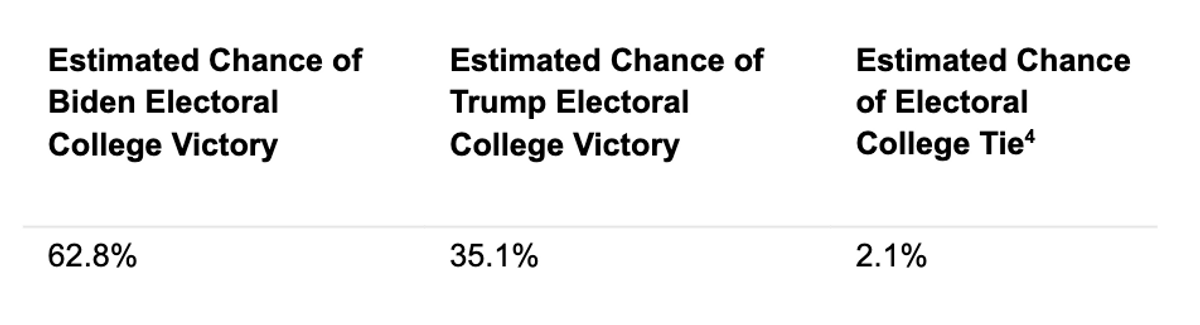
Our first model predicts that Joe Biden will win the election with 273 electoral votes and 52.8% of the national two-party popular vote. However, several tight races in battleground states and a close margin in the Electoral College lead to high levels of uncertainty. With that in mind, this forecast estimates a 62.8% chance of a Biden Electoral College victory, a 35.1% chance of a Trump Electoral College victory, and a 2.1% chance of an electoral tie.

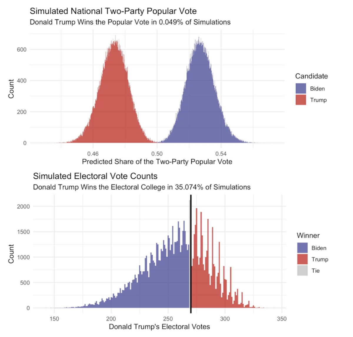
The second model forecasts a much less competitive race: over 10,000 simulated electionis, Trump wins in only 11 cases. Biden wins an average of 389.57 electoral votes and an average of 55.82% of the popular vote, while Trump wins 148.42 electoral college votes and 44.14% of the popular vote on average.

Our first model gives Trump a higher likelihood of victory than most mainstream media outlets, like 538, the New York Times, and the Economist, and our second model aligns pretty well.

Our first, “narrow lead” model uses a mix of economic, demographic, and polling data to predict the probability that a voter will vote for either party within each state. Then, the forecast applies these probabilities to the relevant state’s voting-eligible population to determine that state’s forecasted two-party popular vote. Whichever candidate wins the state most often in 100,000 simulations wins the electoral votes for that state.

The second model uses a similar mix of economic, demographic, and polling data, along with some information about past elections to predict the number of individual votes cast for each candidate in each state. The model has four parts: estimating the turnout in each state, estimating the vote share in each state, estimating a possible national shift in voting behavior, and finally simulating elections based on the estimated values. In this version, voting behavior between states are correlated with one another. For example, a Biden blowout in Pennsylvania would suggest that Biden is doing well in states like Ohio or Michigan.

One major difference that likely explains much of the difference between the two models is data selection: the first model works with individual polls, while the second works with smoothed polling averages. Polling averages, like from FiveThirtyEight, The Economist, or RealClearPolitics, have been remarkably stable throughout the race, while individual polls have fluctuated more over time.

What should be the lesson here? The difference between a very tight race and a blowout is slim. Because of the distribution across states of support for each candidate, Trump has an edge in the electoral college compared to his popular vote share, so a relatively small, systematic polling error in Trump’s favor can make the race really close. However, if the polling is close to reality, or if there’s an error in Biden’s favor, then we will be heading towards a blowout election.

Forecast #1: A Tight Electoral Race

This forecast uses polling numbers as of 3 PM EST on 11/1/2020. See the full forecast and complete Election Analysis blog here.

Overview

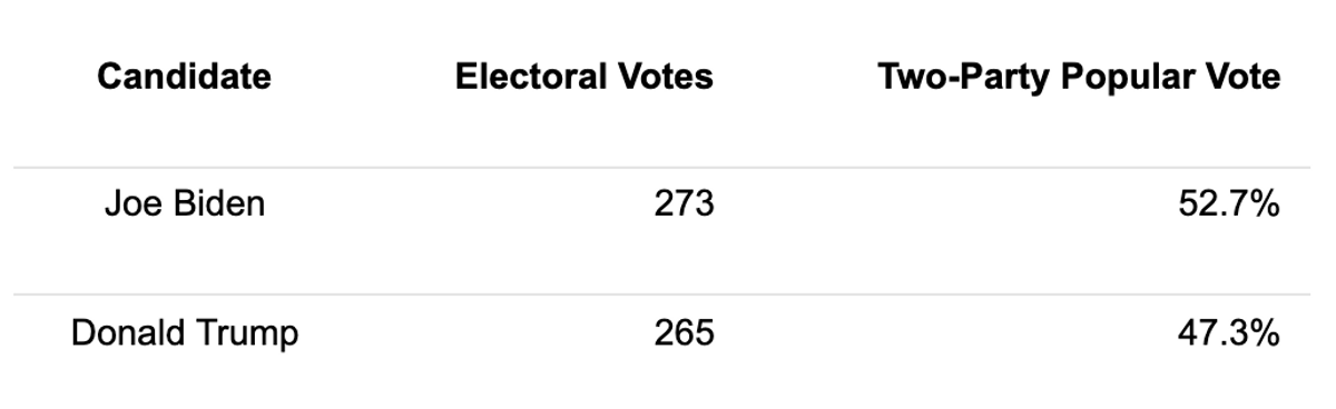
This forecast predicts that Joe Biden will win a popular vote victory of 52.7% with a narrow Electoral College majority of 273 votes compared to Donald Trump’s 265 votes. However, the model projects a high level of uncertainty in several battleground states. As a result, the Electoral College could easily swing to a Trump victory or further in Biden’s favor. In terms of uncertainty, this forecast gives Joe Biden a 62.8% chance of a Joe Biden Electoral College victory, a 35.1% chance of a Donald Trump Electoral College victory, and a 2.1% chance of an electoral tie.

Model Description and Methodology

In this forecast, a binomial logistic model predicts the state-by-state probabilities that an individual will vote for either party, using a combination of polling, economic, demographic, and incumbency data [1].

To gauge public opinion, the model includes average state-level polls [2] in the final 4 weeks before the election. Election-year Q1 GDP growth captures the state of the economy, and the incumbency term accounts for the incumbent advantage. Since past elections serve as excellent predictors for future elections, the forecast includes a term for the difference between Democratic and Republican state-level two-party vote share in the previous election. Lastly, demographic variables [3] –the change in the state’s Black population, age 20-30 population, and age 65+ population–capture the impact of shifting demographics on election outcomes. To produce the 2020 predictions, I applied the coefficients for each of these terms to each states’ data points for this year.

2020 Prediction

This model predicts a narrow Biden victory in the Electoral College, with a much larger margin in the popular vote:

This table contains all state-level predictions of the two-party popular vote.

Uncertainty Around Prediction

Any model, including this one, has a near-zero probability of predicting the exact outcome of an election. However, forecasts provide insights into the range of possible election outcomes and the surrounding uncertainty.

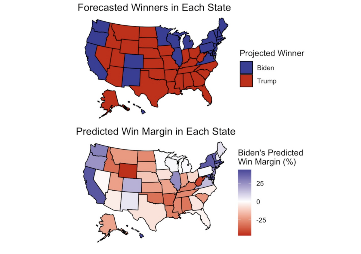
As visible in the map of Joe Biden’s predicted win margin, this forecast anticipates close elections in many states, making a Biden landslide possible in the Electoral College if several of Trump’s close states flip to blue. On the contrary, Trump could win the Electoral College if some of the slightly blue states flip to red. How can we quantify the uncertainty with this forecast?

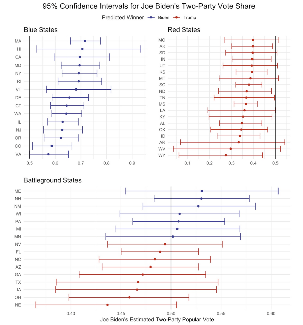
Confidence intervals serve as a helpful tool to measure statistical uncertainty. The below plot displays 95% confidence intervals for Joe Biden’s two-party vote share in each state. If a state’s interval does not contain 50%, then the forecast estimates with 95% confidence that the specified candidate will win that state’s two-party vote:

Moving away from estimated vote share, the remaining probabilities in this section do not represent vote share estimates; rather, these probabilities represent each candidate’s chance of victory. From 100,000 election simulations, this model gives Joe Biden a 62.8% chance of winning the Electoral College and Donald Trump a 35.1% chance of winning the Electoral College, with a 2.1% chance of an electoral tie [4]:

However, Donald Trump has a much smaller chance of winning the national popular vote:

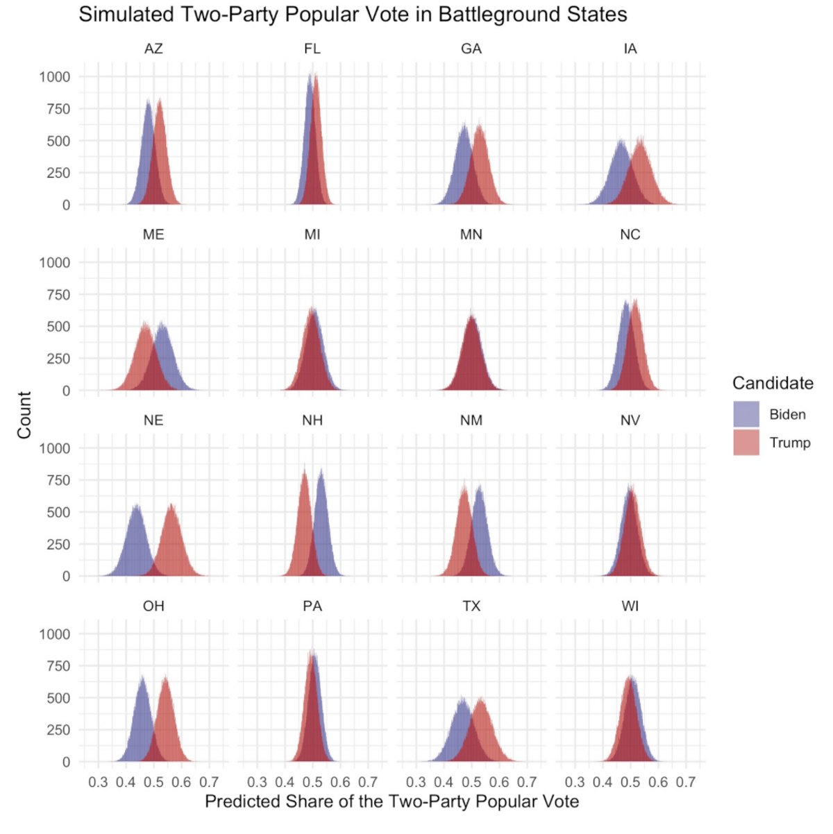
Luckily for Trump, the national popular vote does not matter if he can reach 270 Electoral College votes via statewide victories. While the forecast has a narrow Joe Biden victory as the point prediction, either candidate could reasonably win most of the battleground states. The below graph illustrates the high levels of uncertainty in battleground states, with both candidates winning a reasonable number of the 100,000 simulations in most of these states:

According to this model, the closest battleground races are fairly evenly split between the two candidates. However, these states could all easily swing in Donald Trump’s favor, giving him the Electoral College victory while still losing the popular vote. If one of Minnesota, Michigan, or Florida flip and the other states remain the same, Donald Trump will win the Electoral College. On the other hand, Nevada, Florida, North Carolina, and Iowa could easily all vote for Biden, giving him a much larger Electoral College victory than estimated by the forecast’s point prediction. For a more detailed look at each candidate’s state-level win probabilities, this table lists all states and corresponding levels of uncertainty.

Model Limitations

While this forecast performed quite well in the leave-one-out cross-validation and makes reasonable state-by-state predictions, it also has several limitations:

• This model does not account for Washington D.C. However, D.C. has a history of voting heavily Democratic, making it extremely likely to vote Democrat in this election. For this reason, Washington D.C.’s 3 electoral votes were added to Joe Biden’s Electoral College tally after allocating the votes from the 50 states.
• Due to the structure of the available data, this model treats Maine and Nebraska as winner-take-all states. However, these two states follow the congressional district method and can split their votes between candidates.
• The combined data [5] for this model only dates back to 1992, which only allows for the model to fit itself with data from 7 previous elections. However, each state counts as an individual observation, increasing the total number of observations to 350. 105, 112, and 133 observations fit the blue, battleground, and red models, respectively.
• This model independently varies voter turnout and probabilities for each simulation [6]. A more sophisticated model would introduce some correlation between subgroups such as demographics, COVID deaths, or partisan alignment. For example, low turnout among suburban women in Wisconsin would likely accompany low turnout among suburban women in Minnesota. While this forecast does simulate instances with lower-than-predicted probabilities of voting for either party within each state, the probability of voting for Biden in Wisconsin in a single simulation has no bearing on the probability of voting for Biden in Minnesota.
• To set a rule for how I classified states, I divided states into blue, red, and battleground states using the 2020 classifications by the New York Times. Unfortunately, this method does not account for the ideological evolution of states over time. For example, Texas reliably voted Republican in all other elections from 1992-2016, but the New York Times classifies as a “battleground state” for 2020. Ideally, I would have used historical Texas data to construct the “red state” model. If I did that, however, I would either have to (a) make judgment calls for each of the remaining 49 states in each of the 7 elections, or (b) set some other arbitrary rule for the year-by-year classification of states. In the end, I elected to follow the imperfect but uniform method of classifying states by their 2020 status.

Conclusion

This model predicts a narrow Democratic victory with a 273 to 265 Electoral College majority and approximately 52.7% of the two-party popular vote. However, the close state-level vote margins, especially in battleground states, increase the level of uncertainty.

Due to the close margins in several battleground states, the Electoral College could easily swing in the direction of a Trump victory or a Biden landslide. For example, if Joe Biden wins Michigan, Nevada, Texas, or any other state with a narrow victory projected for Trump, Biden could win far more than his projected 273 votes. However, if Trump wins New Hampshire, Nebraska, Pennsylvania, Wisconsin, or any other states projecting an extremely narrow Biden victory, he could easily tip the electoral scale in his favor. This forecast gives Joe Biden a 62.8% chance of a Joe Biden Electoral College victory, a 35.1% chance of a Donald Trump Electoral College victory, and a 2.1% chance of an electoral tie.

Forecast #2: A Blowout

This forecast uses polling numbers as of 6 PM EST on 11/1/2020. See the full forecast and complete Election Analysis blog here.

Overview

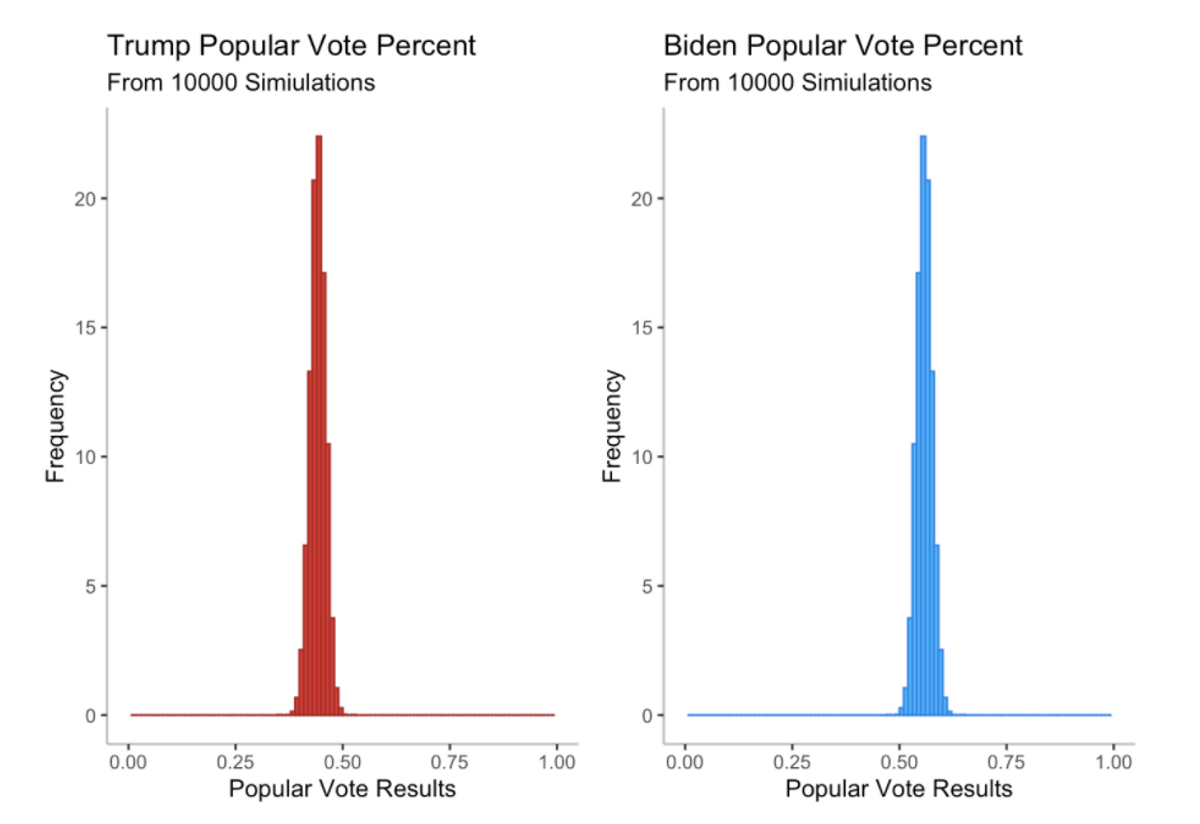
On average, this model predicts that Donald Trump will lose his re-election campaign in dramatic fashion, only winning an average of 148.42 electoral college votes and only 44.14% of the popular vote, while Joe Biden wins handily with 389.57 electoral college votes and an average of 55.82% of the popular vote. In addition, if we look at the winners in the 10,000 individual simulations, Trump only wins in 11 cases, all times when he happens to win the popular vote.

Model Overview and Data

There are four components of this model:

1. Estimating turnout in each state.

2. Estimating vote share for each candidate in each state.

3. Estimating nation wide vote swings.

4. Simulating the election based on the estimated parameters.

Turnout is estimated via a poisson regression on a state by state basis. Vote share for each candidate is estimated using a binomial regression, predicting the fraction of voters that each candidate will win. National swings for each candidate come from the mean and variance of polling errors for each candidate in the past seven elections.

Data for this model comes from a number of sources, which are described in greater detail here. In short, data comes from five categories: polling data, economic data, demographic data, indicators for party and state, and lagged versions of the other four forms of data. The key element is polling data. For the 2020 polling data, I used FiveThirtyEight’s state level polling averages, rather than individual polls. Because they remove a lot of the noise from individual polls, this produces an extremely stable forecast. Polling averages have shown this race as extremely, extremely stable.

The final step in this model is to actually simulate elections, via a probabilistic process. Simulation of each election proceeds as follows:

• Turnout for each state is generated with a draw from a poisson distribution, with the mean as the predicted turnout in that state.
• Vote shares for each candidate are generated with draws from a multivariate normal distribution [7].
• National swings in behavior are generated with draws from a stable distribution for each candidate [8].
• Votes in each state, for each candidate, are drawn from a binomial distribution with the number of trials being the turnout in the state, and the probability of success being the vote share for each candidate plus the national swing.

Results

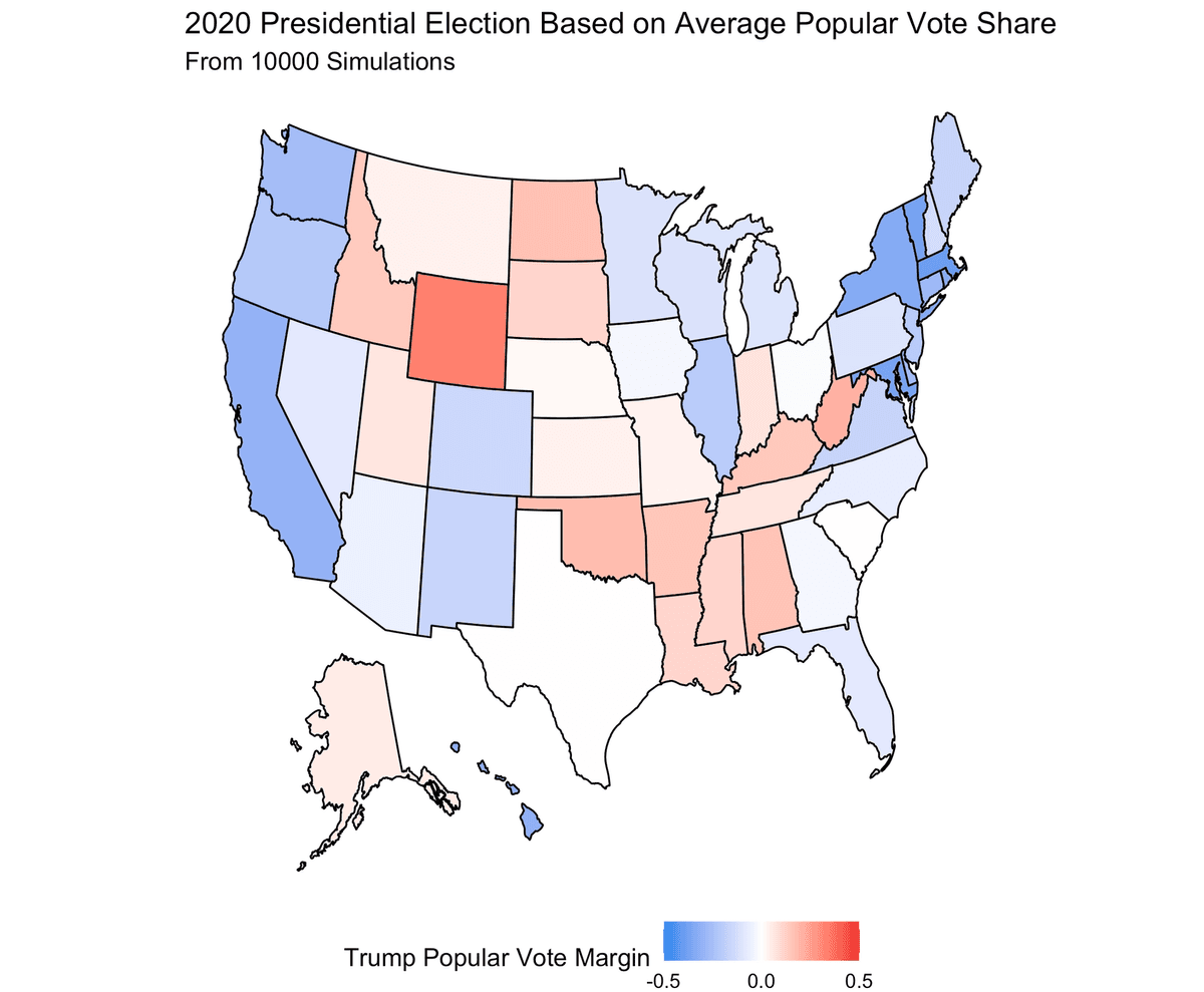
After simulating the election 10,000 times, we can look at the results. We primarily look at the average outcomes across trials. Looking at the average vote shares in each state gives the following map, showing a Biden blowout.

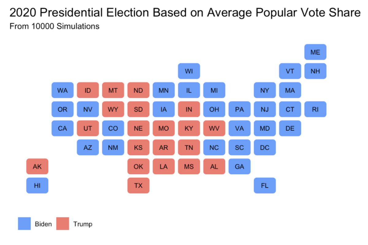
On average, Biden wins South Carolina, Georgia, and Ohio, three states that are only likely to go for Biden in a landslide election. The distribution of electoral college results from each election tells a similar story. 

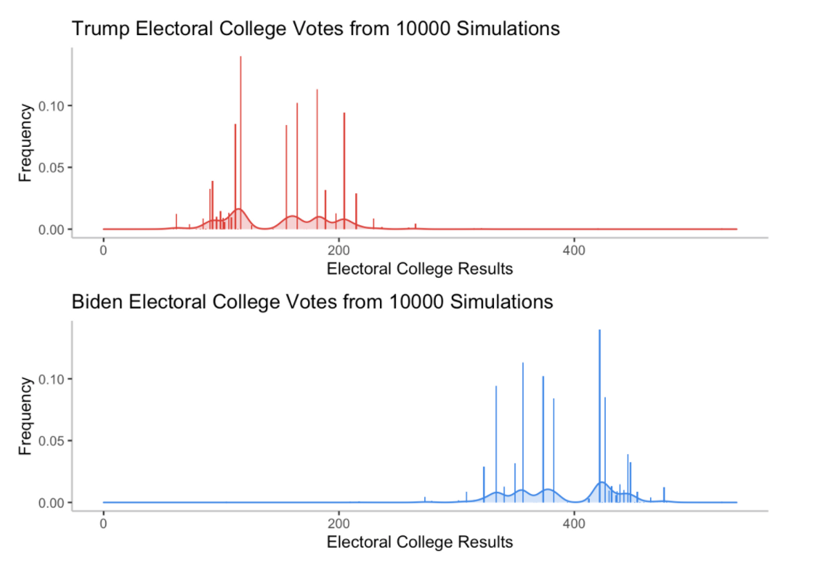
One of the most frequent outcomes is a landslide victory for Biden where he wins 445 electoral college votes, a historic blowout. On the flipside, Trump only wins very, very slim few elections in this simulation, all narrowly. The distribution of the popular vote again tells the story of a lopsided victory. Trump only wins the election when he wins the popular vote, which is an extremely rare occurrence.  

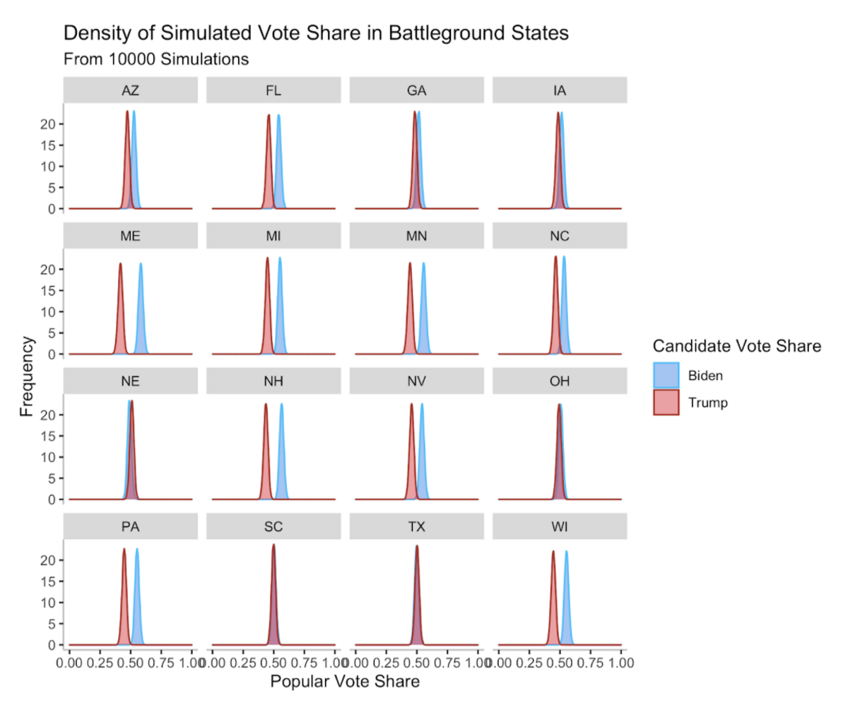
The most informative story from these results is looking at the map of the average vote share margins. Biden wins South Carolina by the slimmest margins on average, and just barely loses Texas as well. One thing to note is that the actual vote shares in many states are much, much closer than these results would indicate. We can look at the density of vote shares for both candidates in a number of battleground states [9]. In many of the key states, the density plots of the popular vote shares at a state level have significant overlap, suggesting that many state elections are quite close. However, because of state to state correlation, overwhelmingly tip the balance in Biden’s favor.  For example, a blowout Biden victory in Pennsylvania means that Biden likely performed well in Ohio, leading to the overall certainty of the model.  It also speaks to Biden having many more paths to 270 electoral votes: he could lose a close state like Ohio and still have enough electoral votes to win.

Model Limitations

There’s a lot going on in this model, and it’s certainly not perfect. While it performed well in leave-one-out validation on a year by year basis for predicting the mean turnout and mean vote shares, the full model was not validated out of sample.

One regret of this model is that the state to state correlation was not fine tuned. State to state correlation is notoriously difficult to get right. In an ideal world, with more time, I would have spent a lot of time fitting the model on previous elections, using it as a way to do out of sample validation. It would be interesting to see how this model performs with data that do not suggest a blowout election.

In a sense, including both variance at the state and national level is double counting variance in the data. Variance in a model at the national level is a direct function of variance at the state level. However, in the uncertain times brought on by COVID-19 and one candidate actively trying to discredit the election results, I decided that increasing the overall variance seems reasonable.

Another note is that this model seems to understate the value of the electoral college - other models do have the possibility of a electoral college and popular vote victor split, which did not occur here.

Conclusions

All in all, this model gives Biden an extremely high chance of victory, which does make sense given the national environment. As noted previously, the polling averages in states have been extraordinarily stable throughout the entire political process, which forms the backbone of the certainty in this model. This model is quite certain of the victory, but everyone should remember that events with small probabilities do happen occasionally, no matter how small the probability is. For example, the roughly 0.1% chance that my model gives Trump is roughly the chance of three randomly selected people all being left handed.

What this model suggests is that for Donald Trump to win re-election, he needs a massive polling error in his favor, or he needs courts to allow him to conduct extra-legal shenanigans that throw out votes. One final thing to remember is this: all models are wrong, but some models are useful. Undoubtedly, this model will be wrong in the exact votes, but it can still tell us that Biden has a very, very good chance of victory.

Footnotes

[1] All data for this model is publicly available online. While many online sources host the data used in this model, the data for the 2020 state-level polls came from FiveThirtyEight, and the national GDP growth numbers came from the US Bureau of Economic Analysis.

[2] State-level polling in 2016 did quite a poor job of forecasting the election outcomes. Since this forecast uses state polls as the variable for public opinion, I aimed to exclude heavily biased or inaccurate polls where possible. To do this, I utilized FiveThirtyEight’s pollster ratings, which assigns grades ranging from A+ to D- to each poll. SurveyMonkey is one of only two pollsters with a rating of D-, but the platform issues the most polls out of anyone–nearly ten times as much as the second most prolific pollster. This pairing of low quality and high quantity makes SurveyMonkey polls incredibly problematic. To account for this, I applied an aggressive weighting scheme in an attempt to “crowd out” the low-rated polls. In calculating the polling averages, I counted A-rated polls 40 times, B-rated polls 20 times, C-rated polls 10 times, and D-rated polls 1 time each. Some states have a shortage of high-rated polls, which does not allow me to exclude low-quality polls altogether. This weighting scheme allows me to use the same technique for every state.

[3] I only had state-level demographic data for the years 1990-2018, so I used the 2018 state-level demographic numbers to produce each party’s 2020 vote count projections. The change of the state’s demographics, as used in the model, accounts for the difference from the previous year’s percent composition of that state’s population. For example, if Alabama’s population was 75% white in 1990 but 74.8% white in 1991, the change in the white population for 1991 would be 0.2%.

[4] This counts the proportion of times that neither candidate received at least 270 electoral votes. In the case of a tie, the House of Representatives would decide the winner of the presidential election.

[5] I could only find state-level demographic data dating back to 1990. Since this model uses state-level demographic variables, it could only fit itself with data from presidential elections from 1992 to the present.

[6] To vary the voting-eligible population (VEP) and the probability of voting for each party, I drew the values from a normal distribution. For the VEP, I used a normal distribution centered at each state’s VEP in 2016 and used a standard deviation of 1.25 times the standard deviation of the VEP in all years from 1980-2016. I multiplied the standard deviation by 1.25 because there will likely be more variability in turnout numbers this year; turnout could decrease in some states as a result of COVID-19 or issues with mail-in ballots, but turnout could also increase, as seen in historic early voting turnout in Texas. To simulate fluctuations in the probability of voting for each party, I took the absolute value of a draw from a normal distribution centered at the predicted probability for 2020 with a standard deviation equivalent to that party’s standard deviation of the two-party popular vote in the last three elections (2008-2016) within the respective state.

[7] A natural choice for vote share would be beta distributions, as we want a probability of voting for a particular candidate, and the values are bounded between zero and one. However, in this case, the parameters of the beta distributions with corresponding means and variances are quite large, meaning that it can be well approximated by a normal distribution. This approximation is key, because it gives a very convenient way to have vote probabilities that are correlated between states, using the multivariate normal distribution. We can calculate a covariance matrix in two steps: first, building a similarity matrix that tells us how similar each state is to one another, using all of the non-categorical data from the vote share model. The key detail of this similarity matrix is that values are between -1 and 1. Values near 1 indicate high similarity (or correlation), and negative values indicate that states are very dissimilar. We can then scale this makeshift correlation matrix by standard deviations in the polls over the past three weeks to get a covariance matrix. The standard deviations in the polling averages that I use are quite small, suggesting a very stable race, and therefore a relatively small amount of uncertainty.

[8] I intentionally picked stable distributions because they are "fat-tailed," meaning that events farther from the mean, holding variance fixed, happen more frequently than in a normal distribution. This choice is meant to introduce a potentially large amount of polling error, and therefore variance into the model. Something to note is that these terms are independent for each candidate: both Biden and Trump could have polling errors in their favor in this model. This fits with the fact that both parties tend to outperform their polls, by 2.40 and 2.11 points for Democrats and Republicans respectively.

[9] Using the same definition as before, but swapping out South Carolina because it’s quite close in this model, for New Mexico, which was a blowout.